
Bestand:Savitzky-golay pic gaussien bruite.svg

Afmetingen van deze voorvertoning van het type PNG van dit SVG-bestand: 610 × 407 pixels Andere resoluties: 320 × 214 pixels | 640 × 427 pixels | 1.024 × 683 pixels | 1.280 × 854 pixels | 2.560 × 1.708 pixels.
Oorspronkelijk bestand (SVG-bestand, nominaal 610 × 407 pixels, bestandsgrootte: 43 kB)
| Dit is een bestand van Wikimedia Commons. Onderstaande beschrijving komt van de beschrijving van het bestand daar. |
Beschrijving
| Beschrijving |
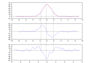
English: Savitzky-Golay algorithm (3rd degree polynomial, 9 points) applied on a gaussian peak with random noise: smoothing (top), first derivation (middle), second derivation (bottom).
The dashed lines highlight the zeros of the second dérivative (inflection points of the peak) and its minimum (top of the peak). Created with Scilab, processed with Inkscape.Français : Application de l'algorithme de Savitzky-Golay sur un pic gaussien bruité (polynôme de degré 3, 9 points) : lissage (haut), dérivée (milieu), dérivée seconde (bas).
Les traits pointillés mettent en évidence l'annulation de la dérivée seconde (points d'inflexion du pic) et son minimum (sommet du pic). Créé avec Scilab, retravaillé avec Inkscape. |
| Datum | |
| Bron | Eigen werk |
| Auteur | Christophe Dang Ngoc Chan |
| SVG ontwikkeling |  English: English version by default.
Français : Version française, si les préférences de votre compte sont réglées (voir Special:Preferences). De broncode van dit SVG-bestand is deugdelijk. Deze vectorafbeelding is gemaakt met Scilab This file uses embedded text. |
| Broncode | (1) File generateur_pic_bruit.sce : generates a set of data and save it in the file noisy_gaussian_peak.txt.
SciLab code// **********
// Constants and initialisation
// **********
clear;
chdir("mypath/");
// parameters of the noisy curve
paramgauss(1) = 60; // height of the gaussian curve
paramgauss(2) = 3; // "width" of the gaussian curve
var=0.01; // variance of the noise normal law
nbpts = 100 // nombre of points
halfwidth = 3*paramgauss(2) // range for x
step = 2*halfwidth/nbpts;
// **********
// Fonctions
// **********
// gaussian peak
function [y] = gauss(A, x)
// A(1) : height of the peak
// A(2) : "width" of the peak
y = A(1)*exp(-x.^2/A(2));
endfunction
// **********
// Main program
// **********
// Generation of data
for i=1:nbpts
x = step*i - halfwidth;
X(i) = x;
Y(i) = gauss([paramgauss], x) + rand(var, "normal");
end
// Saving the data
write ("noisy_gaussian_peak.txt", [X, Y])
(2) File savitzkygolay.sce : processes the data.
Data// **********
// Constants and initialisation
// **********
clear;
clf;
chdir("mypath/")
// smoothing parameters :
width = 9; // width of the sliding window (number of pts)
poldeg = 3; // degree of the polynomial
// **********
// Functions
// **********
// Convolution coefficients
function [a]=convolcoefs(m, d)
// m : width of the window (number of pts)
// d : degree of the polynomial
l = (m-1)/2; // half-width of the window
z = (-l:l)'; // standardised abscissa
J = ones(m,d+1);
for i = 2:d+1
J(:,i) = z.^(i-1); // jacobian matrix
end
A = (J'*J)^(-1)*J';
a = A(1:3,:);
endfunction
// smoothing, determination of the first and second derivatives
function [y, yprime, ysecond] = savitzkygolay(X, Y, width, deg)
// X, Y: collection of data
// width: width of the window (number of pts)
// deg: degree of the polynomial
n = size(X, "*");
l = floor(width/2);
step = (X($)-X(1))/(n - 1);
y = Y;
yprime=zeros(Y);
ysecond=yprime;
a = convolcoefs(width, deg);
a(2,:) = 1/step*a(2,:);
a(3,:) = 2/step^2*a(2,:);
for i = 1:width
Ymat(i, :) = Y(i: n-width+i)';
end
solution = a*Ymat;
y = solution(1, :)';
yprime = solution(2, :)';
ysecond = solution(3, :)';
endfunction
// **********
// Main program
// **********
// data reading
data = read("noisy_gaussian_peak.txt", -1, 2)
Xinit = data(:,1);
Yinit = data(:,2);
//subplot(3,1,1)
//plot(Xdef, Ydef, "b")
// Data processing
[Ysmooth, Yprime, Ysecond] = savitzkygolay(Xinit, Yinit, width, poldeg);
// Display
offset = floor(width/2);
nbpts = size(Xinit, "*");
X1 = Xinit((offset+1):(nbpts-offset)); // removal of non-smotthed points
subplot(3,1,1)
plot(Xinit, Yinit, "b")
plot(X1, Ysmooth, "r")
subplot(3,1,2)
plot(X1, Yprime, "b")
subplot(3,1,3)
plot(X1, Ysecond, "b")
(3) When the sampling step is not constant, i.e. xi - xi - 1 varies, then it is possible to determine the polynomial by multi-linear regression. Text// **********
// Constants and initialisation
// **********
clear;
clf;
chdir("mypath\")
// smoothing parameters
width = 9; // width of the sliding window (number of pts)
// **********
// Functions
// **********
// 3rd degree polynomial
function [y]=poldegthree(A, x)
// Horner method
y = ((A(1).*x + A(2)).*x + A(3)).*x + A(4);
endfunction
// regression with the 3rd degree polynomial
function [A]=regression(X, Y)
// X, Y: column vectors of "width" values ;
// determines the polynomial of degree 3
// a*x^2 + b*x^2 + c*x + d
// by regression on (X, Y)
XX = [X.^3; X.^2; X];
[a, b, sigma] = reglin(XX, Y);
A = [a, b];
endfunction
// smoothing, determination of the first and second derivatives
function [y, yprime, ysecond] = savitzkygolay(X, Y, larg)
// X, Y: collection of data
n = size(X, "*");
l = floor(larg/2); // halfwidth
y=Y;
yprime=zeros(Y);
ysecond=yprime;
for i=(l+1):(n-l)
intervX = X((i-l):(i+l),1);
intervY = Y((i-l):(i+l),1);
Aopt = regression(intervX', intervY');
x = X(i);
y(i) = poldegthree(Aopt,x);
// Yfoo=poldegthree(Aopt,intervX);
// subplot(3,1,1) ; plot(intervX, Yfoo, "r")
yprime(i) = (3*Aopt(1)*x + 2*Aopt(2))*x + Aopt(3); // Horner
ysecond(i) = 6*Aopt(1)*x + 2*Aopt(2);
end
endfunction
// **********
// Main program
// **********
// data reading
data = read("noisy_gaussian_peak.txt", -1, 2)
Xinit = data(:,1);
Yinit = data(:,2);
//subplot(3,1,1)
//plot(Xdef, Ydef, "b")
// Data processing
[Ysmooth, Yprime, Ysecond] = savitzkygolay(Xinit, Yinit, width);
// Display
offset = floor(width/2);
nbpts = size(Xinit, "*");
vector1 = (offset+1):(nbpts-offset); // suppresion des points non-lissés
X1 = Xinit(vector1);
Y0 = Yliss(vector1)
Y1 = Yprime(vector1);
Y2 = Ysecond(vector1);
subplot(3,1,1)
plot(Xinit, Yinit, "b")
plot(X1, Y0, "r")
subplot(3,1,2)
plot(X1, Y1, "b")
subplot(3,1,3)
plot(X1, Y2, "b")
|
Licentie
Ik, de auteursrechthebbende van dit werk, maak het hierbij onder de volgende licenties beschikbaar:

|
Toestemming wordt verleend voor het kopiëren, verspreiden en/of wijzigen van dit document onder de voorwaarden van de GNU-licentie voor vrije documentatie, versie 1.2 of enige latere versie als gepubliceerd door de Free Software Foundation; zonder Invariant Sections, zonder Front-Cover Texts, en zonder Back-Cover Texts. Een kopie van de licentie is opgenomen in de sectie GNU-licentie voor vrije documentatie. |
Dit bestand is gelicenseerd onder de Creative Commons-licenties Naamsvermelding-Gelijk delen 3.0 Unported, 2.5 Algemeen, 2.0 Algemeen en 1.0 Algemeen.
- De gebruiker mag:
- Delen – het werk kopiëren, verspreiden en doorgeven
- Remixen – afgeleide werken maken
- Onder de volgende voorwaarden:
- naamsvermelding – U moet op een gepaste manier aan naamsvermelding doen, een link naar de licentie geven, en aangeven of er wijzigingen in het werk zijn aangebracht. U mag dit op elke redelijke manier doen, maar niet zodanig dat de indruk wordt gewekt dat de licentiegever instemt met uw werk of uw gebruik van zijn werk.
- Gelijk delen – Als u het werk heeft geremixt, veranderd, of erop heeft voortgebouwd, moet u het gewijzigde materiaal verspreiden onder dezelfde licentie als het oorspronkelijke werk, of een daarmee compatibele licentie.
U mag zelf één van de licenties kiezen.
Bestandsgeschiedenis
Klik op een datum/tijd om het bestand te zien zoals het destijds was.
| Datum/tijd | Miniatuur | Afmetingen | Gebruiker | Opmerking | |
|---|---|---|---|---|---|
| huidige versie | 9 nov 2012 15:07 | | 610 × 407 (43 kB) | Cdang | dashed line to highlight the inimum of the second derivative |
| 9 nov 2012 12:50 |  | 610 × 407 (43 kB) | Cdang | {{Information | description = {{en|1=Savitzky-Golay algorithm (3<sup>rd</sup> degree polynomial, 9 points) applied on a gaussian peak with random noise: smoothing (top), first derivation (middle), second derivation (bottom). Created with Scilab, proce... |
Bestandsgebruik
Dit bestand wordt op de volgende pagina gebruikt:
Globaal bestandsgebruik
De volgende andere wiki's gebruiken dit bestand:
- Gebruikt op es.wikipedia.org
- Gebruikt op fr.wikipedia.org
- Gebruikt op fr.wikibooks.org